


By Manusha Rao
You’ll have seen that markets typically stay calm for weeks after which swing wildly for a number of days. That’s volatility in motion. It measures how a lot costs transfer—and it’s an enormous deal in buying and selling and investing as a result of it displays danger. However right here’s the catch: estimating volatility is not simple.
A 2% drop typically sparks extra headlines than a 2% acquire. That’s uneven volatility—and it is what conventional fashions miss.
Enter the GJR-GARCH mannequin!
Conditions
This weblog focuses on volatility forecasting utilizing the GJR-GARCH mannequin, with a sensible Python implementation based mostly on the NIFTY 50 index. It explains the idea of uneven volatility, the way it differs from the standard GARCH mannequin, and gives instruments for evaluating forecast high quality by visualizations and diagnostics.
To grasp and apply the GJR-GARCH mannequin successfully, it is necessary to begin with the fundamentals of time sequence evaluation. Start with Introduction to Time Collection to get conversant in pattern, seasonality, and autocorrelation. For those who’re exploring how deep studying compares to conventional fashions, learn Time Collection vs LSTM Fashions for a conceptual comparability.
Since GARCH and GJR-GARCH fashions depend on stationary time sequence, research Stationarity to discover ways to put together your knowledge. Improve this information by studying The Hurst Exponent for insights into long-term reminiscence in time sequence and Imply Reversion in Time Collection for understanding mean-reverting conduct—typically linked with volatility clusters.
You must also be conversant in the ARMA household of fashions, that are foundational to ARIMA and GARCH. For this, discuss with the ARMA Mannequin Information and its companion weblog ARMA Implementation in Python. Lastly, to understand the terminology and idea behind GARCH, the Quantra glossary entries on GARCH and Volatility Forecasting utilizing GARCH are important sources.
On this weblog, we are going to discover the next:
Distinction between GARCH and GJR-GARCH fashions
The GARCH mannequin captures volatility clustering however assumes that optimistic and detrimental shocks have a symmetric impact on future volatility. In distinction, the GJR-GARCH mannequin accounts for asymmetry by giving extra weight to detrimental shocks, which displays the leverage impact generally noticed in monetary markets. Why? As a result of concern drives quicker and stronger reactions than optimism in monetary markets.
GJR-GARCH introduces a further parameter that prompts when previous returns are detrimental. This makes it extra appropriate for modelling real-world inventory knowledge, the place dangerous information sometimes causes larger volatility.
For instance, throughout the COVID-19 market crash in March 2020, the NIFTY 50 noticed sharp declines and sudden spikes in volatility pushed by panic promoting proven beneath.
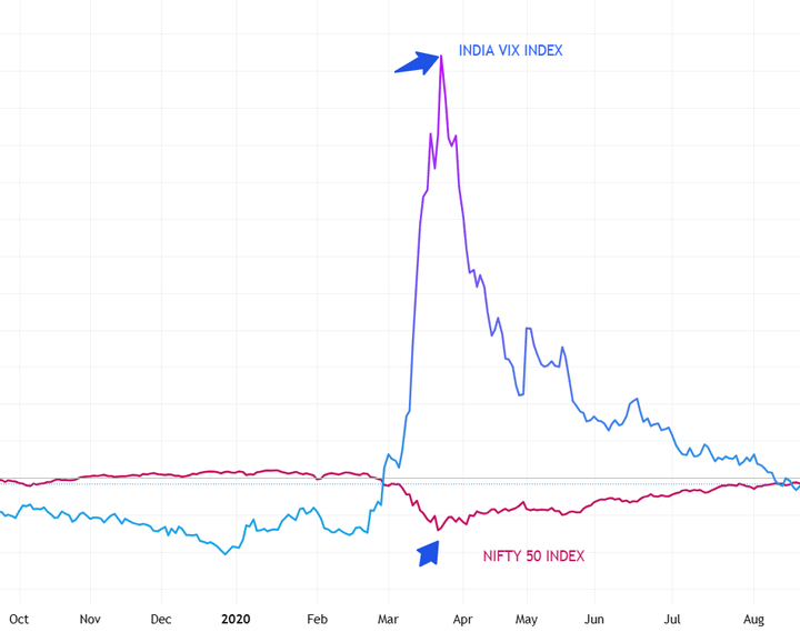
Supply: TradingView
A GARCH mannequin would understate this asymmetry, whereas GJR-GARCH captures the heightened volatility following detrimental shocks extra precisely. Total, GJR-GARCH is a extra versatile and practical extension of the usual GARCH mannequin.
A short have a look at the GARCH mannequin
The GARCH (Generalized Autoregressive Conditional Heteroskedasticity) mannequin is a well-liked statistical software for forecasting monetary market volatility. Developed by Tim Bollerslev in 1986 as an extension of the ARCH mannequin, GARCH captures the tendency of volatility to cluster over time—that means durations of excessive volatility are usually adopted by durations of excessive volatility, and durations of calm are adopted by extra durations of calm.
In essence, the GARCH mannequin assumes that as we speak’s volatility relies upon not solely on previous squared returns (as in ARCH) but in addition on previous volatility estimates. This makes it particularly helpful for modelling time sequence knowledge with altering variance, resembling asset returns.
The final equation for a GARCH(p, q) mannequin, which fashions conditional variance, is:

σ2t: Represents the conditional variance of the time sequence at time ‘t’.
ω: A continuing time period representing the long-run or common variance.
Σ(αi * ε2t−i): The ARCH element, capturing the impact of previous squared errors on the present variance.
Σ(βj * σ2t−j): The GARCH element, capturing the impact of previous conditional variances on the present variance.
Word: GARCH(1,1) is the best type of the GARCH mannequin:
σ2t = ω + α1 ε2t−1 + β1 σ2t−1
With solely three parameters (fixed, ARCH time period, and GARCH time period), it is easy to estimate and interpret—excellent for monetary knowledge the place too many parameters will be unstable.
Introduction to the GJR-GARCH mannequin
The GJR-GARCH mannequin, proposed by Glosten, Jagannathan, and Runkle (1993), is an extension of the usual GARCH mannequin designed to seize the uneven results of reports on volatility.
The GJR-GARCH(1,1) formulation is given by:
σ2t = ω + α1 ε2t−1 + γ ε2t−1 It−1 + β1 σ2t−1
The place,
γ : Represents the extra influence of detrimental shocks (leverage impact)
ε2t−1 It−1
: Represents the indicator perform that prompts when the earlier return shock is detrimental
Interpretation:
When the earlier shock
εt−1
is optimistic:σt2 = ω + α εt−12 + β σt−12
When the earlier shock
εt−1
is detrimental:σt2 = ω + (α + γ) εt−12 + β σt−12
So, detrimental shocks improve volatility extra by the quantity
γ
Now that we perceive the GJR-GARCH mannequin formulation and its instinct, let’s implement it in Python. We’ll use the arch bundle, which provides a easy but highly effective interface to specify and estimate GARCH-family fashions. Utilizing historic NIFTY 50 returns knowledge, we’ll match a GJR-GARCH(1,1) mannequin, generate rolling volatility forecasts, and consider how properly the mannequin captures market conduct, particularly throughout turbulent durations.
Volatility Forecasting on NIFTY 50 Utilizing GJR-GARCH in Python
Step 1: Import the mandatory libraries
The tqdm library is used to indicate a progress bar when your code is doing one thing that takes time — like working a loop with plenty of steps.
It helps you see how a lot is completed and the way a lot is left, so that you don’t must guess in case your code remains to be working or caught.
Step 2: Obtain NIFTY50 knowledge
Right here we’re utilizing NIFTY 50 knowledge from 2020 to 2025.

Subsequent, calculate the every day log returns and specific in proportion phrases. Fashions like GARCH work higher when the enter numbers are usually not too tiny (like 0.0012), as very small values could make it more durable for the optimizer to converge throughout mannequin becoming.
Step 3: Specify the GJR-GARCH mannequin
To mannequin a GJR-GARCH mannequin in Python,the arch bundle is used. Use Pupil’s t-distribution for residuals, which captures fats tails typically noticed in monetary returns. Be at liberty to make use of the distribution that most accurately fits your buying and selling wants or knowledge distribution.
Right here,
p = 1
Variety of lags of previous squared returns (ARCH time period)
o = 1
Variety of lags for asymmetry time period – this permits the GJR-GARCH (or GARCH with leverage impact)
q = 1
Variety of lags of previous variances (GARCH time period)
Step 4: Match the mannequin
The output is as follows:

The ARCH time period (alpha[1]), which measures the influence of previous shocks, is critical on the 5% stage, although comparatively small (0.0123).The GARCH time period (beta[1]) is excessive at 0.9052, implying that volatility is extremely persistent over time.The leverage impact (gamma[1] = 0.1330) is critical, confirming the presence of asymmetry—detrimental shocks improve volatility greater than optimistic ones, a typical characteristic in fairness market knowledge.The estimated levels of freedom (nu = 7.6) for the Pupil’s t-distribution counsel the information displays fats tails, justifying the selection of this distribution to seize excessive returns extra precisely.
Step 5: Residual diagnostics
This block of code is for residual diagnostics after becoming your GJR-GARCH mannequin. It helps you visually assess how properly the mannequin has captured volatility dynamics.
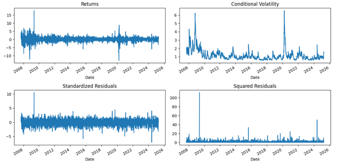
The GJR-GARCH mannequin performs properly in capturing volatility dynamics throughout main market occasions, particularly durations of monetary misery. Notable spikes in conditional volatility are noticed throughout the 2008 world monetary disaster and the 2020 COVID-19 pandemic. The asymmetry element (gamma) performs a key position right here, amplifying volatility predictions in response to detrimental returns—mirroring real-world investor conduct the place concern and dangerous information drive sharper market reactions than optimism.
Step 6: Make rolling forecasts of volatility
A extra sensible method to forecast volatility is to make one-step-ahead predictions utilizing data accessible as much as time t, after which replace the mannequin in actual time as every new knowledge level turns into accessible (i.e., as t progresses to t+1, t+2, and so forth.). In easy phrases, every day we incorporate the newest noticed return to forecast the following day’s volatility.
Right here we take practice the mannequin on 500 days of previous returns, to forecast 1-day forward volatility, repeated every day.
Now you’ll need to evaluate GARCH’s 1-day forecast to some observable precise volatility.
The standard technique is to compute realized every day volatility as a rolling normal deviation.
Nonetheless, if you happen to’re forecasting for 1 day, the realized volatility it is best to ideally evaluate it to is:
the precise return (i.e., squared return of the following day), or a smoothed proxy like a 5-day rolling normal deviation (if you wish to take away noise).
As illustrated within the plot beneath, durations of elevated market uncertainty, resembling mid-2024, exhibit vital spikes within the 1-day forward forecasted volatility, reflecting heightened danger notion. Conversely, calmer durations like early 2023 present decreased volatility expectations. This method allows merchants and danger managers to adaptively alter publicity and hedging methods in response to anticipated market situations.
The GJR-GARCH mannequin proves particularly priceless for its skill to react sensitively to draw back shocks. It’s a strong software for short-term volatility forecasting in index-level knowledge just like the NIFTY 50 or inventory knowledge.

Now allow us to verify the correlation between the realized and forecasted volatility.
Output:
Correlation between Forecasted and Realized Volatility: 0.7443
The noticed correlation of 0.74 between the 5-day rolling realized volatility and the GJR-GARCH forecasted volatility signifies that the mannequin successfully captures the dynamics of market volatility.
Particularly, the GJR-GARCH mannequin, which accounts for uneven responses to optimistic and detrimental shocks (i.e., volatility reacts extra to detrimental information), aligns properly with the precise realized volatility. A powerful correlation like this implies that the mannequin can forecast durations of excessive or low volatility in a directionally correct method.
Conclusion
Market volatility isn’t simply numbers—it displays human psychology. The GJR-GARCH mannequin goes a step past conventional volatility estimators by recognizing that concern has a stronger market influence than optimism. By modelling this behaviour explicitly, it gives a extra correct and behaviourally sound option to forecast volatility in varied property.
Subsequent Steps
When you’re comfy with the GARCH household, you may transfer on to extra advanced volatility modeling methods. A superb subsequent learn is Time-Various-Parameter VAR (TVP-VAR), which introduces fashions that deal with stochastic volatility and structural modifications over time.
You too can discover ARFIMA fashions for dealing with long-memory processes, that are widespread in monetary market volatility. Understanding these fashions will show you how to create extra strong, adaptable forecasting techniques.
To develop efficient buying and selling methods, transcend modeling. Mix your GJR-GARCH insights with sensible strategies from Technical Evaluation to detect tendencies and momentum, use Buying and selling Danger Administration to guard in opposition to losses, discover Pairs Buying and selling for market-neutral methods, and perceive Market Microstructure to account for execution and liquidity dynamics.
Lastly, for a structured and complete journey into algorithmic buying and selling, think about enrolling within the Govt Programme in Algorithmic Buying and selling (EPAT). EPAT covers superior matters resembling stationarity, ACF/PACF, ARIMA, ARCH, GARCH, and extra, with sensible coaching in Python technique improvement, statistical arbitrage, and alternate knowledge. It’s the proper subsequent step for these prepared to use their quantitative abilities in actual markets.
File within the obtain:
GJR GARCH Python Pocket book
Login to Obtain
Disclaimer: All investments and buying and selling within the inventory market contain danger. Any resolution to position trades within the monetary markets, together with buying and selling in inventory or choices or different monetary devices is a private resolution that ought to solely be made after thorough analysis, together with a private danger and monetary evaluation and the engagement {of professional} help to the extent you imagine essential. The buying and selling methods or associated data talked about on this article is for informational functions solely.