


Entrance Operating in Nation ETFs, or The best way to Spot and Leverage Seasonality
Understanding seasonality in monetary markets requires recognizing how predictable return patterns may be influenced by investor habits. One underexplored facet of that is the affect of front-running—the place merchants anticipate seasonal traits and act early, shifting returns ahead in time. We now have already explored seasonality front-running in commodities, inventory sectors, and disaster hedge portfolios. Our new analysis examines whether or not this phenomenon extends to nation ETFs, an asset class the place seasonality has been much less studied. By making use of a front-running technique to a dataset of nation ETFs, we establish alternatives to capitalize on seasonal results earlier than they totally materialize. Our findings point out that pre-seasonality drift is strongest in commodities however stays current in nation ETFs, providing a possible edge in portfolio development. Finally, our research highlights how front-running seasonality can improve ETF investing, offering an extra layer of market timing past conventional trend-following approaches.
Introduction
Seasonality is a well-documented phenomenon in monetary markets, the place sure belongings exhibit recurring patterns in returns based mostly on time-based components equivalent to months, quarters, or financial cycles. It generally seems in commodity markets (Dealer’s Information to Entrance-Operating Commodity Seasonality), inventory sectors (Entrance-Operating Seasonality in US Inventory Sectors) or disaster hedge portfolios (Seasonality Patterns within the Disaster Hedge Portfolios).
As soon as tradable belongings change into accessible, they’re topic to entrance operating—buyers anticipating seasonal traits start accumulating positions earlier than the anticipated seasonality manifests. This entrance operating impact can create worth drifts, shifting returns ahead in time and doubtlessly diminishing or reshaping the unique seasonal sample. Whereas not all belongings expertise this impact, it’s removed from uncommon. Understanding these dynamics will help buyers establish when and the place seasonality is being priced in early, providing alternatives to capitalize on market inefficiencies.
On this research, we examine whether or not this phenomenon extends to a different phase of the market—market ETFs. We study the habits of those ETFs with a deal with seasonality and, following the method of the beforehand talked about research, goal to assemble a front-running technique that successfully leverages seasonal patterns.
Knowledge
On this evaluation, our dataset encompass month-to-month information from 23 nation ETFs, particularly: SPY – SPDR S&P 500 ETF Belief, EWU – iShares MSCI United Kingdom ETF, EWG – iShares MSCI Germany ETF, EWQ – iShares MSCI France ETF, EWI – iShares MSCI Italy ETF, EWD – iShares MSCI Sweden ETF, EWN – iShares MSCI Netherlands ETF, EWP – iShares MSCI Spain ETF, EWK – iShares MSCI Belgium ETF, EWL – iShares MSCI Switzerland ETF, EWC – iShares MSCI Canada ETF, EWJ – iShares MSCI Japan ETF, EWW – iShares MSCI Mexico ETF, EWM – iShares MSCI Malaysia ETF, EWA – iShares MSCI Australia ETF, EWS – iShares MSCI Singapore ETF, EWY – iShares MSCI South Korea ETF, EWT – iShares MSCI Taiwan ETF, EWZ – iShares MSCI Brazil ETF, EWH – iShares MSCI Hong Kong ETF, EZA – iShares MSCI South Africa ETF, FXI – iShares China Massive-Cap ETF, and INDY – iShares India 50 ETF.
Most of those ETFs had been launched in 1996, the second largest group in 2000; subsequently, after the 12 months 2000, now we have historic information for practically all ETFs. Solely EZA, FXI, and INDY had been launched later, in 2003, 2004, and 2009, respectively. To maximise the size of our analysis interval, we didn’t wait till 2009. As an alternative, we used the 12 months 2000 as the place to begin for our evaluation, and the final 3 ETFs had been included steadily after their inception. In different phrases, we tried to make a trade-off between information availability and the variety of ETFs within the preliminary portfolio. The latest information used was from February 2025.
Month-to-month efficiency information had been utilized in all calculations. Fundamental efficiency traits in tables are introduced as follows: the notation perf represents the annual return of the technique, st dev stands for the annual customary deviation, max dd is the utmost drawdown, adusted Sharpe Ratio is calculated because the ratio of perf to st dev and adjusted Calmar Ratio because the ratio of perf to max dd.
Methodology
As talked about within the first paragraph, this research focuses on seasonality, which we goal to leverage in making a worthwhile technique. Given the supply of tradable belongings, we consider front-running is an acceptable method. The process is simple – if we’re assured that an asset performs nicely in a particular month, shopping for it one month earlier, earlier than most buyers do, may be more practical, as their later purchases drive the worth increased.
And now, we are able to transfer on to the technique itself. On the finish of every month, we utilized a cross-sectional method to seasonality, rating the efficiency of all included ETFs based mostly on their returns from the month T-11 (e.g., on the finish of March, investments for April had been ranked based mostly on their efficiency in Might of the earlier 12 months). This rating was performed relative to the opposite ETFs within the choice. Primarily based on these rankings, we invested in a specific variety of top-performing ETFs for the next month.
However what number of ETFs ought to we embrace in our portfolio? We determined to depend on acquired information, and for robustness functions, we included all important picks. Subsequently, we examined a number of thresholds: vigintile (prime 5%), decile (prime 10%), quintile (prime 20%), quartile (prime 25%), tercile (prime 33%), and half (50%). This implies we utilized the front-running technique to the highest 1 to 11 ranked investments.
Within the subsequent step, we constructed a benchmark – an equally weighted common of all 23 ETFs. Moreover, we included an equally weighted common of the 11 front-running methods, choosing the highest 1 to 11 ETFs with the best efficiency within the front-running months. Now, we’re lastly able to assess the profitability of our technique.


As we are able to see within the graph in Determine 1, for nearly the complete interval, practically all front-running methods and their common outperformed the benchmark. There may be one exception: the front-running technique, which selects only one ETF, which has skilled a major downturn since 2019. All different methods, and thus the common 1-11, simply outperformed the benchmark.
Nonetheless, methods positioned in the midst of our examined pattern achieved probably the most favorable outcomes. Evidently it’s not a good suggestion to be too concentrated (choosing simply the 1 or 2 ETFs). It’s additionally not a good suggestion to be overly diversified (because the front-running sign is then too diluted amongst too many ETFs). The candy spot is to choose between 3-8 ETFs (so the highest quintile, quartile, or tercile of ETFs based mostly on the front-running seasonality sign). So, within the subsequent step, we retained solely the methods based mostly on the highest 3 to prime 8 ETFs and averaged them out to construct a last front-running technique. Let’s assess whether or not we made the best resolution.

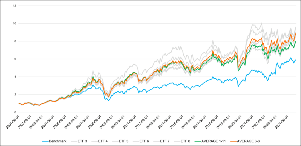

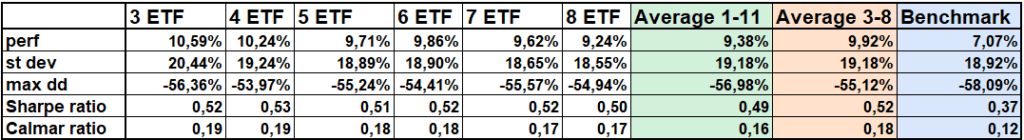
As anticipated, the shortened choice simply outperformed not solely the benchmark but additionally the broader common. Subsequently, we suggest adopting the common of shortened choice as the ultimate technique, much like our method within the research Can Margin Debt Assist Predict SPY’s Progress & Bear Markets?. We take into account the marginally increased outcomes of some methods to have low credibility and to be unlikely to persist in the long term. As a result of imply reversion impact, we favor diversifying our bets throughout all methods to keep up a extra secure mannequin. The ultimate resolution, after all, stays with the reader.
Conclusion
The power of the pre-seasonality drift is determined by the underlying belongings. We observe that it’s strongest in commodities, the place we first recognized it. Whereas the impact is current in different asset courses, it’s weaker because of the dominance of different basic components. For instance, in equities, the general robust constructive drift performs a serious function, as shares are likely to rise on common, whereas commodities don’t exhibit the identical long-term upward pattern. Regardless of this, now we have discovered a approach to improve funding methods in nation ETFs by implementing an method that evenly allocates capital throughout six front-running methods, choosing 3 to eight ETFs based mostly on the front-running seasonality sign every month. This demonstrates that the front-running seasonality idea stays relevant past commodities.
Writer: Sona Beluska, Junior Quant Analyst, Quantpedia
Are you searching for extra methods to examine? Join our e-newsletter or go to our Weblog or Screener.
Do you need to be taught extra about Quantpedia Premium service? Test how Quantpedia works, our mission and Premium pricing provide.
Do you need to be taught extra about Quantpedia Professional service? Test its description, watch movies, evaluation reporting capabilities and go to our pricing provide.
Are you searching for historic information or backtesting platforms? Test our checklist of Algo Buying and selling Reductions.
Or comply with us on:
Fb Group, Fb Web page, Twitter, Linkedin, Medium or Youtube
Share onLinkedInTwitterFacebookConsult with a pal


")


